

- お役立ち記事
- Basics and practical points of time series analysis using Python

Basics and practical points of time series analysis using Python

目次
Understanding Time Series Analysis
Time series analysis is a statistical method used to analyze a sequence of data points collected over time.
These data points can represent anything that varies over time, such as stock prices, weather patterns, or a patient’s vital signs.
The primary goal of time series analysis is to understand the underlying pattern and forecast future values.
One of the unique aspects of time series data is its temporal ordering.
Unlike other types of data, where observations are usually considered independent, time series data points are dependent on their historical values.
This dependency must be considered when constructing models, making the analysis process more complex but also more rewarding.
Types of Time Series Data
Time series data can fall into various categories based on patterns and characteristics.
It’s crucial to identify these properties to choose the right analysis techniques.
1. **Trend**: A trend is a long-term increase or decrease in the data. It’s the overall direction that the data points move over a longer period.
2. **Seasonality**: Seasonal variations are patterns that repeat at regular intervals. For example, retail sales often peak during holiday seasons.
3. **Cyclic**: These are long-term fluctuations that are not fixed and differ from seasonal patterns. Cycles can last several years, unlike the more regular seasonal patterns.
4. **Noise**: Random variations that do not follow any pattern are considered noise. Noise can obscure the true understanding of trends and patterns.
Understanding these components can help in choosing the right model for time series analysis.
Introduction to Python for Time Series Analysis
Python provides a rich ecosystem of libraries that simplify time series analysis.
The combination of its simplicity and power makes Python a preferred choice for data analysts and scientists.
Some essential Python libraries for time series analysis include:
– **Pandas**: Offers powerful data structures for data manipulation and analysis. Useful for reading and handling time series data.
– **NumPy**: Provides support for mathematical computations, fundamental for many analysis tasks.
– **Matplotlib and Seaborn**: Used for data visualization. They can plot time series data to help visualize trends and seasonal patterns.
– **Statsmodels and SciPy**: Contain tools for statistical modeling and hypothesis testing, useful for implementing various time series models.
– **Scikit-learn**: While primarily used for machine learning, it offers tools for preprocessing data and feature selection that can apply to time series.
Practical Steps to Perform Time Series Analysis
Performing time series analysis involves several steps.
Here’s a guide to follow when analyzing time series data using Python:
Step 1: Data Importation and Exploration
The first step is to acquire the data. The data can be imported using Pandas, which efficiently handles time-stamped indices:
“`python
import pandas as pd
data = pd.read_csv(‘time_series_data.csv’, parse_dates=[‘date’], index_col=’date’)
print(data.head())
“`
After importing the data, it’s crucial to explore it. Exploring helps understand the structure of the data and identify any potential issues, such as missing values.
Step 2: Data Preprocessing
Preprocessing involves cleaning the data.
This step includes handling missing values, detecting and adjusting outliers, and transforming the data if necessary.
Missing values can be filled using several methods, including interpolation or using specific techniques like forward filling:
“`python
data.fillna(method=’ffill’, inplace=True)
“`
Step 3: Visualizing the Data
Visualization is a powerful tool for uncovering hidden insights in the data.
Using Matplotlib and Seaborn, you can plot the data to identify the trend, seasonal components, and any irregular patterns.
“`python
import matplotlib.pyplot as plt
plt.figure(figsize=(10, 6))
plt.plot(data.index, data[‘value’])
plt.title(‘Time Series Data’)
plt.xlabel(‘Date’)
plt.ylabel(‘Value’)
plt.show()
“`
Step 4: Decompose the Time Series
Decomposition is a technique that breaks down a time series into its underlying trend, seasonal, and noise components.
This helps in understanding and interpreting the series.
Statsmodels provides a handy function for seasonal decomposition:
“`python
from statsmodels.tsa.seasonal import seasonal_decompose
result = seasonal_decompose(data[‘value’], model=’additive’)
result.plot()
plt.show()
“`
Step 5: Model Selection and Fitting
After decomposing the series and understanding its components, the next step is to fit a model that can capture these patterns for forecasting.
Commonly used models for time series forecasting include:
– **ARIMA (AutoRegressive Integrated Moving Average):** Suitable for univariate series without trends and seasonality after differencing.
– **SARIMA (Seasonal ARIMA):** An extension of ARIMA that supports seasonality.
– **Prophet:** Developed by Facebook, it is robust and adapts to various time series patterns.
Using a simple ARIMA model:
“`python
from statsmodels.tsa.arima.model import ARIMA
model = ARIMA(data[‘value’], order=(5, 1, 0))
model_fit = model.fit()
print(model_fit.summary())
“`
Step 6: Model Evaluation and Forecasting
Evaluate the model’s performance using metrics such as Mean Absolute Error (MAE), Mean Squared Error (MSE), or Root Mean Squared Error (RMSE).
Good evaluation techniques ensure the accuracy of forecasts.
“`python
forecast = model_fit.forecast(steps=10)
print(forecast)
“`
Forecast future values using the fitted model to make informed decisions based on predictions.
Conclusion
Time series analysis is a powerful technique for understanding and forecasting data based on historical values.
Python, with its versatile libraries, provides a comprehensive framework for performing these analyses efficiently.
By exploring the time series data, preprocessing it, visualizing it, and fitting it into models, one can gain deep insights and make accurate predictions.
Whether dealing with financial data, weather patterns, or any sequence of data over time, the analysis techniques discussed above serve as a practical foundation for deriving actionable insights.
この記事の理解を深める
無料ホワイトペーパーをプレゼント
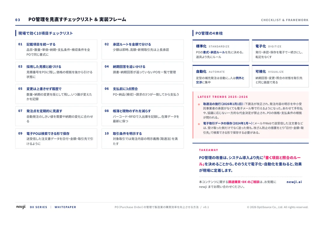
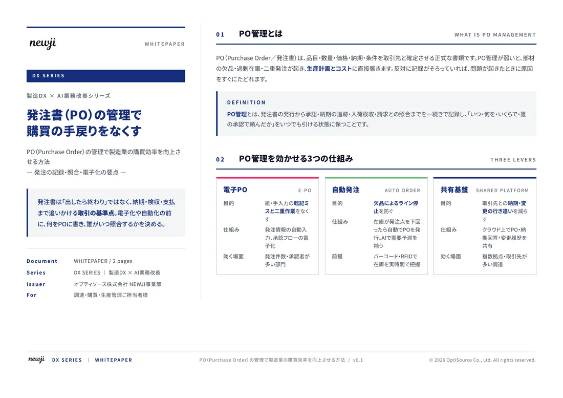
製造業の現場で使える実務資料(PDF)を無料でお届けします。"こんな資料が届きます" ↓ 下のボタンからどうぞ。
FREE DOCUMENT — サービス資料(PDF・無料)
製造業の見積・受発注クラウド
「Newji one」とは
Newji one は、製造業の調達・受発注に特化したクラウド/AIエージェント。見積依頼・発注書作成・進捗管理・承認をひとつの画面に集約し、AIが比較と異常検知を担当。最後の「GO」だけ人が押す仕組みです。
▶ 製造業の見積・受発注クラウド「Newji one」を、資料で見る(PDF・無料)
- 見積〜発注〜納期を一元管理。催促・転記のムダをゼロに
- AIが相見積もり比較と異常検知。あなたは判断だけに集中
- 取引先は「招待」で完全無料。自社コストだけで取引先ごとデジタル化
※ 取引先から招待された企業様は完全無料でご利用いただけます


 NEWJI総研
 OEM/ODM 生産委託
 AI/DX支援
 見積・発注クラウド Newji one
受発注が増えるほど、入力・確認・催促が重くなる。
受発注管理を“仕組み化“して、ミスと工数を削減しませんか。
見積・発注・納期まで一元管理できます。