

- お役立ち記事
- Derivation of Bayes theorem and concrete examples

その単価は妥当か。
AI が根拠付きで分析。
相見積の比較も発注も進捗管理も、ひとつの画面に。

Derivation of Bayes theorem and concrete examples

目次
Understanding Bayes’ Theorem
Bayes’ theorem is a fundamental concept in probability theory and statistics, with wide-ranging applications in fields such as machine learning, data science, and decision-making processes.
At its core, Bayes’ theorem provides a way to update probabilities based on new evidence.
This theorem is named after Thomas Bayes, an 18th-century statistician and minister, who first provided a framework for inductive reasoning.
Bayes’ theorem is particularly useful when dealing with uncertainty and gaining insights from incomplete information.
By understanding its derivation and practical applications, one can effectively utilize it to make informed decisions.
Derivation of Bayes’ Theorem
Bayes’ theorem can be mathematically expressed as:
\[ P(A|B) = \frac{P(B|A) \cdot P(A)}{P(B)} \]
This equation can be broken down to understand its components:
– \( P(A|B) \): The probability of event A occurring, given that event B has occurred.
– \( P(B|A) \): The probability of event B occurring, given that event A has occurred.
– \( P(A) \): The probability of event A occurring independently of the other.
– \( P(B) \): The probability of event B occurring independently of the other.
To derive Bayes’ theorem, let’s start by considering the definition of conditional probability:
\[ P(A|B) = \frac{P(A \cap B)}{P(B)} \]
This equation highlights that the probability of A given B is equal to the joint probability of A and B, divided by the probability of B.
Similarly, we can express:
\[ P(B|A) = \frac{P(A \cap B)}{P(A)} \]
By rearranging this equation, we get:
\[ P(A \cap B) = P(B|A) \cdot P(A) \]
Now, combining both expressions for \( P(A \cap B) \) and substituting, we arrive at Bayes’ theorem:
\[ P(A|B) = \frac{P(B|A) \cdot P(A)}{P(B)} \]
Concrete Examples of Bayes’ Theorem
Bayes’ theorem may seem abstract at first glance, but it can be applied in many practical situations.
Let’s explore a few examples that illustrate its use in real-world decisions.
Example 1: Medical Diagnosis
Imagine a scenario where a doctor is diagnosing a patient for a particular disease.
Let’s say the prior probability \( P(\text{Disease}) \) of a patient having the disease is 1%.
The probability of receiving a positive test result given the patient has the disease \( P(\text{Positive Test}|\text{Disease}) \) is 99%.
Further, the probability of receiving a positive test result even if the patient does not have the disease \( P(\text{Positive Test}|\text{No Disease}) \) is 5%.
The overall probability of a positive test \( P(\text{Positive Test}) \) is:
\[ P(\text{Positive Test}) = P(\text{Positive Test}|\text{Disease}) \cdot P(\text{Disease}) + P(\text{Positive Test}|\text{No Disease}) \cdot P(\text{No Disease}) \]
Thus:
\[ P(\text{Positive Test}) = 0.99 \cdot 0.01 + 0.05 \cdot 0.99 = 0.0594 \]
Now, applying Bayes’ theorem to find the probability that the patient has the disease given a positive test result:
\[ P(\text{Disease}|\text{Positive Test}) = \frac{P(\text{Positive Test}|\text{Disease}) \cdot P(\text{Disease})}{P(\text{Positive Test})} \]
\[ P(\text{Disease}|\text{Positive Test}) = \frac{0.99 \cdot 0.01}{0.0594} \approx 0.1667 \]
This result demonstrates that, despite a positive test, the relatively low prior probability affects the post-test probability significantly.
Example 2: Spam Email Filtering
Consider an email spam filter that uses Bayes’ theorem to determine whether an email is spam or not.
Let’s assume:
– The prior probability of an email being spam \( P(\text{Spam}) \) is 20%.
– The probability that a spam email contains the word “offer” \( P(\text{“Offer”}|\text{Spam}) \) is 70%.
– The probability that a non-spam email contains the word “offer” \( P(\text{“Offer”}|\text{Not Spam}) \) is 10%.
We need to find the probability that an email is spam given that it contains the word “offer”:
\[ P(\text{Spam}|\text{“Offer”}) = \frac{P(\text{“Offer”}|\text{Spam}) \cdot P(\text{Spam})}{P(\text{“Offer”})} \]
First, calculate \( P(\text{“Offer”}) \):
\[ P(\text{“Offer”}) = P(\text{“Offer”}|\text{Spam}) \cdot P(\text{Spam}) + P(\text{“Offer”}|\text{Not Spam}) \cdot P(\text{Not Spam}) \]
\[ P(\text{“Offer”}) = 0.70 \cdot 0.20 + 0.10 \cdot 0.80 = 0.22 \]
Now, apply Bayes’ theorem:
\[ P(\text{Spam}|\text{“Offer”}) = \frac{0.70 \cdot 0.20}{0.22} \approx 0.6364 \]
This probability indicates that if an email contains the word “offer,” there is approximately a 63.64% chance that it is spam.
The Power of Bayes’ Theorem
Bayes’ theorem empowers individuals and systems to make probabilistic inferences based on observed data and prior knowledge.
Its applications extend to various domains, including medical diagnostics, spam filtering, finance, and machine learning.
By continually updating beliefs with new evidence, Bayes’ theorem enables more accurate and data-driven decisions.
Understanding and applying Bayes’ theorem equips you with a valuable statistical tool for navigating uncertainty and making informed predictions.
この記事の理解を深める
無料ホワイトペーパーをプレゼント
製造業の現場で使える実務資料(PDF)を無料でお届けします。"こんな資料が届きます" ↓ 下のボタンからどうぞ。
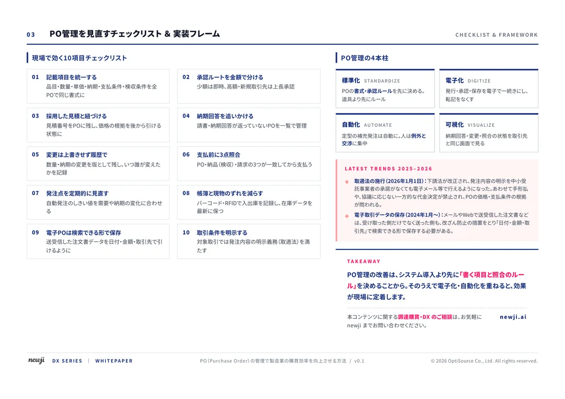
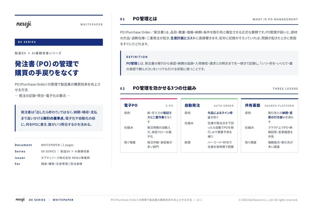
FREE DOCUMENT — サービス資料(PDF・無料)
製造業の見積・受発注クラウド
「Newji one」とは
Newji one は、製造業の調達・受発注に特化したクラウド/AIエージェント。見積依頼・発注書作成・進捗管理・承認をひとつの画面に集約し、AIが比較と異常検知を担当。最後の「GO」だけ人が押す仕組みです。
▶ 製造業の見積・受発注クラウド「Newji one」を、資料で見る(PDF・無料)
- 見積〜発注〜納期を一元管理。催促・転記のムダをゼロに
- AIが相見積もり比較と異常検知。あなたは判断だけに集中
- 取引先は「招待」で完全無料。自社コストだけで取引先ごとデジタル化
※ 取引先から招待された企業様は完全無料でご利用いただけます


 NEWJI総研
 OEM/ODM 生産委託
 AI/DX支援
 見積・発注クラウド Newji one
受発注が増えるほど、入力・確認・催促が重くなる。
受発注管理を“仕組み化“して、ミスと工数を削減しませんか。
見積・発注・納期まで一元管理できます。