A procedure for identifying state equation models without hesitation Continuous system transfer function state equation system identification Transfer function to state equation conversion DC motor example

Introduction to System Identification

System identification is a crucial process in control engineering that involves developing mathematical models of dynamic systems from measured data.
These models help in analyzing, predicting, and controlling system behavior.
In practical scenarios, especially in control system design, it’s essential to identify the state equation models of systems.
This process often begins with the identification of transfer function models, which can then be converted into state space representations.

Understanding Transfer Functions

Transfer functions are mathematical representations of the input-output behavior of linear, time-invariant (LTI) systems.
They are typically represented in the Laplace domain and consist of a ratio of polynomials.
The numerator and denominator polynomials represent the system’s zeros and poles, respectively.

Basic Structure of Transfer Functions

A transfer function, G(s), can be expressed as:

\( G(s) = \frac{N(s)}{D(s)} \)

Where:
– \( N(s) \) is the numerator polynomial
– \( D(s) \) is the denominator polynomial

Transfer functions are particularly useful for understanding system stability, frequency response, and transient response characteristics.

State Equation Models

State equation models are another way to represent dynamic systems, involving a set of first-order differential equations.
They describe the internal state of the system at any given time and provide insight into the dynamics between state variables and outputs.

Formulating State Space Equations

The standard form of a continuous-time state space model is:

\[
\begin{align*}
\dot{x}(t) &= Ax(t) + Bu(t) \\
y(t) &= Cx(t) + Du(t)
\end{align*}
\]

Where:
– \( x(t) \) is the state vector
– \( \dot{x}(t) \) is the derivative of the state vector
– \( u(t) \) is the input vector
– \( y(t) \) is the output vector
– \( A, B, C, D \) are matrices with appropriate dimensions

Conversion from Transfer Function to State Equation

While transfer functions provide a straightforward input-output relationship, the state space representation offers more comprehensive model information.
The conversion from a transfer function to a state space model can be done systematically.

Step-by-Step Conversion Process

1. **Determine System Order**:
– The system order is determined by the degree of the denominator polynomial.

2. **Controllability Canonical Form**:
– Convert the transfer function into the controllability canonical form.
– This form expresses matrices \( A, B, C, \) and \( D \) based on the coefficients of the transfer function polynomials.

3. **Formulate State Matrices**:
– Construct the matrix \( A \) using negative coefficients of the denominator (without the leading coefficient).
– Create the matrix \( B \) as a column vector, usually with a ‘1’ at its topmost position.
– Construct the matrix \( C \) using the numerator coefficients and modifying according to the denominator’s order.
– The matrix \( D \) is typically taken from DC gain or set to zero in the absence of direct gain.

Example: DC Motor System

To illustrate the concept, consider the dynamics of a simple DC motor.
The transfer function of the DC motor can be represented as:

\( G(s) = \frac{K}{(Ls + R)(Js + b) + K^2} \)

Where:
– \( L \) is the inductance
– \( R \) is the resistance
– \( J \) is the inertia
– \( b \) is the damping coefficient
– \( K \) is the motor constant

Identifying the State Equation Model

1. **Identify Poles and Zeros**:
– The poles are derived from the denominator, while zeros are from the numerator.

2. **Canonical State Space Representation**:
– Given that the DC motor transfer function simplifies to second-order, matrices \( A, B, C, \) and \( D \) are derived using the procedure outlined.

3. **Real-World Application**:
– This state space model can be employed to design control systems, such as motor speed or position controllers.
– Simulation tools or numerical methods can simulate system performance, feeding into control design.

Conclusion

In summary, identifying continuous system transfer function models and converting them to state space equations is a fundamental process in dynamic system analysis and control design.
Through systematic steps, engineers can leverage these mathematical models to optimize and control various engineering systems, such as DC motors.
By understanding both transfer function and state space representations, control engineers are better equipped to develop robust, efficient control systems that meet design criteria and performance expectations.

WHITE PAPER

この記事の理解を深める
無料ホワイトペーパーをプレゼント

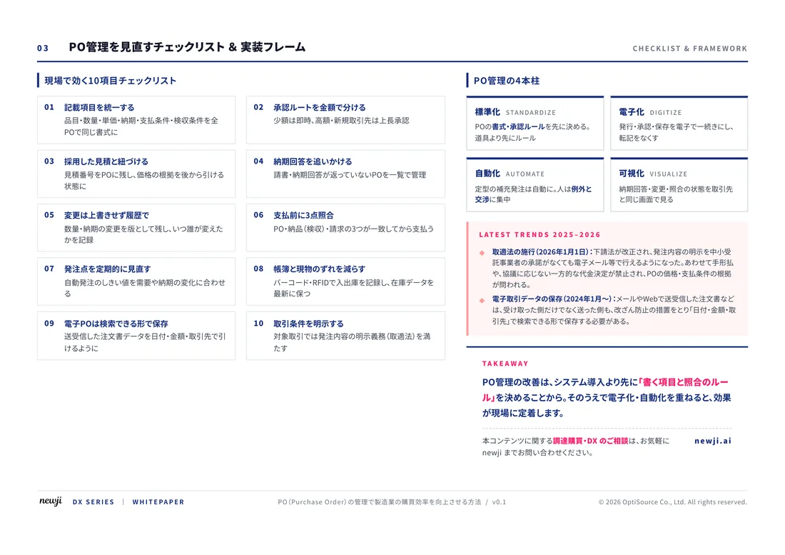
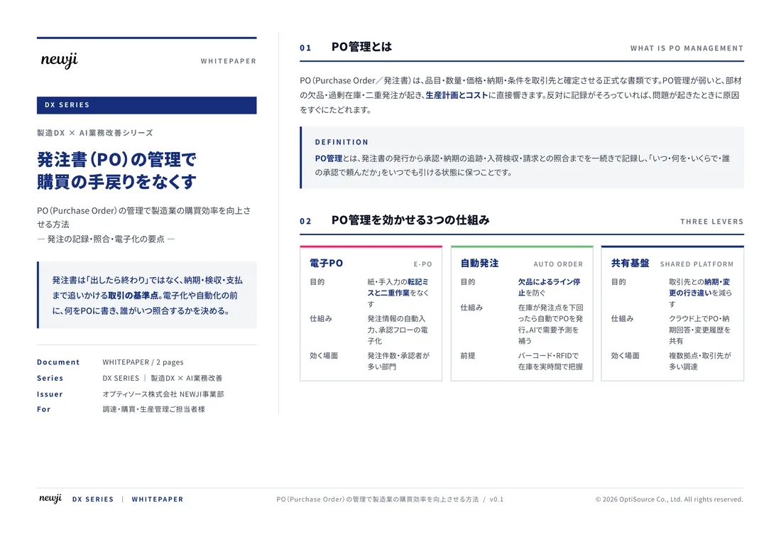
製造業の現場で使える実務資料（PDF）を無料でお届けします。"こんな資料が届きます" ↓ 下のボタンからどうぞ。

🔒 全文は無料ダウンロードで