
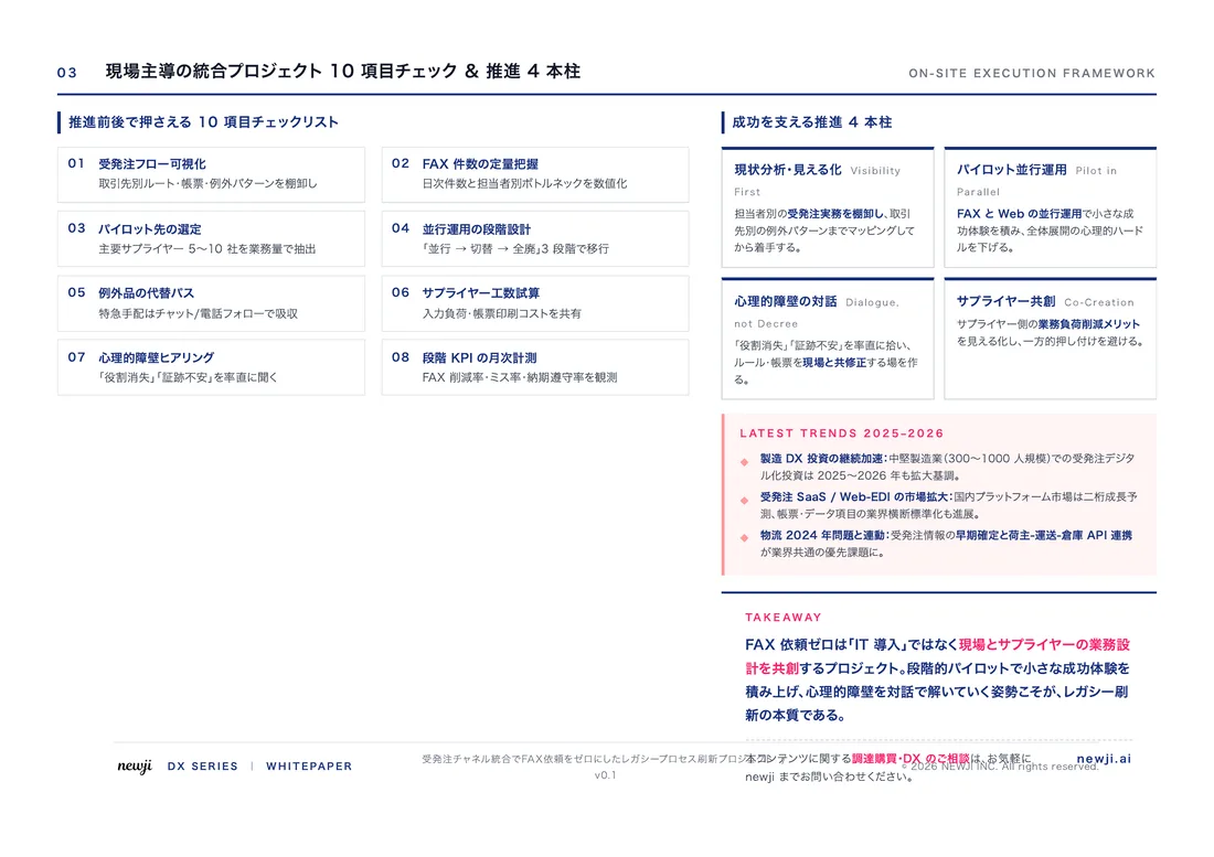
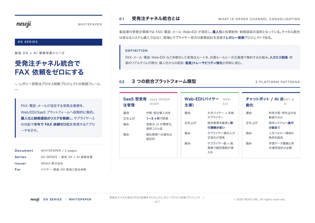
- お役立ち記事
- Transfer function and state equation
スタートアップから大手まで。
調達・受発注をAIで標準化。
相見積比較も進捗管理もAIが下支え。取引先は招待で完全無料。

Transfer function and state equation

目次
Understanding Transfer Function
The concept of a transfer function is pivotal in the field of control systems and engineering.
It represents the relationship between the input and output of a system using mathematical expressions.
Essentially, a transfer function provides a mathematical model that helps in predicting system behavior in response to various inputs.
This is particularly useful in designing and analyzing systems to ensure they perform as intended.
A transfer function is expressed in terms of Laplace transforms, which convert differential equations into algebraic equations.
This conversion greatly simplifies the process of system analysis by focusing on system dynamics in the frequency domain rather than in the time domain.
The transfer function is generally denoted by \( G(s) \) and is expressed as the ratio of the Laplace transform of the output \( Y(s) \) to the Laplace transform of the input \( X(s) \):
\[ G(s) = \frac{Y(s)}{X(s)} \]
where \( s \) is the complex frequency parameter.
Components of Transfer Function
A transfer function is typically represented as a fraction of two polynomials, which includes:
– The numerator polynomial that represents the zeros of the system.
– The denominator polynomial that represents the poles of the system.
Zeros are the frequency values where the system output becomes zero despite having a finite input, whereas poles are the frequency values that make the system output tend to infinity.
Understanding these components is integral for predicting how the system responds to different frequencies and for determining its stability.
Applications of Transfer Functions
Transfer functions play a crucial role in various applications:
1. **Control System Design**: Engineers use transfer functions to design controllers that ensure systems behave in a desired way.
By assessing the system response, they can decide on appropriate compensations to achieve specific performance objectives.
2. **System Stability Analysis**: By examining the position of poles and zeros, engineers can determine the stability of a system.
A system is generally stable if all poles are located in the left half of the complex plane.
3. **Frequency Response Analysis**: Transfer functions enable engineers to understand how systems react to different frequency inputs.
Bode plots and Nyquist plots, which are graphical representations, are widely used for this purpose.
Exploring State Equations
The state equation is another important concept in control systems.
Unlike transfer functions, which describe the system in the frequency domain, state equations provide a time-domain representation of the system.
State equations describe the evolution of the system’s state variables—a set of variables that capture the system’s conditions at any given time.
These equations consist of two main components:
1. **State Equation**: It describes how the state of the system changes over time with the following form:
\[ \dot{x}(t) = Ax(t) + Bu(t) \]
where:
– \( \dot{x}(t) \) is the derivative of the state vector \( x(t) \),
– \( A \) is the state matrix describing the dynamics,
– \( B \) is the input matrix linking the input vector \( u(t) \) to the system.
2. **Output Equation**: It relates the state and input to the output as follows:
\[ y(t) = Cx(t) + Du(t) \]
where:
– \( y(t) \) is the output vector,
– \( C \) is the output matrix,
– \( D \) is the feedthrough (or direct transmission) matrix.
Uses of State Equations
State equations offer several benefits and are used in various contexts:
– **Modeling Complex Systems**: They are particularly useful for modeling systems with multiple inputs and outputs (MIMO systems), providing a unified framework for analysis.
– **Observability and Controllability**: State-space models facilitate the analysis of observability (how well internal states can be inferred from outputs) and controllability (whether the internal states can be manipulated by inputs).
– **Simulation and Real-Time Control**: In computer simulations and real-time control systems, state-space representations are preferred as they are well-suited for digital implementations.
Connecting Transfer Function and State Equation
While transfer functions and state equations are different representations, they are interconnected.
For linear time-invariant (LTI) systems, it is possible to convert a transfer function to a state-space model and vice versa.
– **From Transfer Function to State Equation**: Transforming a transfer function into state-space form involves determining matrices \( A \), \( B \), \( C \), and \( D \) from the given polynomials of numerator and denominator.
This process provides insights into the system’s internal state dynamics.
– **From State Equation to Transfer Function**: Converting state equations to a transfer function is achieved by taking the Laplace transform of the state and output equations, which results in:
\[ G(s) = C(sI – A)^{-1}B + D \]
where \( I \) is the identity matrix.
These transformations are vital for system analysis as they allow engineers to leverage the strengths of both representations depending on the task at hand.
Conclusion
Transfer functions and state equations are key tools in the realm of control systems.
Each serves a distinct purpose and provides unique insights into system behavior.
Transfer functions excel in frequency-domain analysis and are ideal for simple single-input, single-output systems.
Conversely, state equations provide a powerful framework for describing complex systems in the time domain, allowing for detailed analysis and control design.
Understanding the interrelationship between these two representations is crucial for effective system modeling and analysis, aiding in the development of stable and efficient systems across various engineering applications.
この記事の理解を深める
無料ホワイトペーパーをプレゼント
製造業の現場で使える実務資料(PDF)を無料でお届けします。"こんな資料が届きます" ↓ 下のボタンからどうぞ。
PRODUCT — 製造業向け 調達・受発注クラウド
この記事の課題、
newji で解決しませんか?
newji は、製造業の調達・受発注に特化したクラウド/AIエージェント。見積依頼・発注書作成・進捗管理・承認をひとつの画面に集約し、AIが比較と異常検知を担当。最後の「GO」だけ人が押す仕組みです。
- 見積〜発注〜納期を一元管理。催促・転記のムダをゼロに
- AIが相見積もり比較と異常検知。あなたは判断だけに集中
- 取引先は「招待」で完全無料。自社コストだけで取引先ごとデジタル化
※ 取引先から招待された企業様は完全無料でご利用いただけます
関連記事
-

強化学習・深層強化学習の基礎と実装プログラミング
-

Metal Matrix Composite (MMC):革新的な素材が製造調達に与える影響とは?
-

「Metal Matrix Composite (MMC)で製造業の営業力を強化するための革新的戦略」
-

Manufacturing Innovations Enabled by Digital Twin Technology
-
技術移転 (Technology Transfer)の方法とサプライチェーンでの活用法
-

The Importance of Factory Layout Planning! Space Utilization for Efficient Production
